Volume 13, Issue 1, 1999
Investigating Parameter Time Invariance or Stationarity with Excel Graphics
- Lisa A Wilder
- Bowling Green State University
Articles in recent issues of CHEER have shown how spreadsheets can aid in teaching economics. Some papers have shown how spreadsheet applications have been particularly useful in macroeconomics (
Paetow, 1998,
Thomas, 1996, and
Goddard, Romilly and Tavakoli, 1995).
1 In addition,
Judge, 1990 includes many spreadsheet applications suitable for introductory economics. This paper shows how we can use a spreadsheet to explore the assumption of stationarity in econometrics, macroeconomics or more specialized courses.
A fundamental assumption in model building is that the behavior of the phenomena to be studied is stationary or invariant over time. This stationarity is also a crucial assumption in empirical studies so that the collected data represent repeated observations of a particular population. In order for reliable model solutions or estimates of population parameters to be found, a series must continue to retain the same basic underlying data structure.
Today, many studies of economic phenomena include the ideas of non-stationarity and the use of cointegration. However, introducing this material to students at either the undergraduate or graduate level is a difficult task or, at best, a time consuming one. This paper will demonstrate spreadsheet graphs can be used to show students the implications of non-stationarity on model parameters.
Section 1 of this paper discusses the benefits of using these techniques. Section 2 discusses the estimation method and shows how to construct a spreadsheet to explore the time invariance properties. Section 3 demonstrates the estimation techniques with a common example, the consumption function.
1. Examining Stationarity in Economics Courses
The Benefits of Introducing Stationarity through Spreadsheets
Including spreadsheets in economics courses and utilizing the spreadsheet to explore estimator properties over time can serve several purposes. These include:
- The use of spreadsheets satisfies the increased need for curriculum integration. One way integration can be accomplished is through the use of statistics and computers in the economics classroom. Often students in advanced (and sometimes introductory) economics classes have been exposed to statistical techniques such as regression. I find that many students do not retain enough statistical knowledge to successfully implement regression analysis nor do they see the connection between statistics and other courses. Using estimation in economics can demonstrate the importance of statistics and can provide additional practical experience.
- Students learn actively in an interactive environment.
- Students gain increased capability and confidence with spreadsheet software.
- Using the computer in economics classes may enhance student motivation and morale.Often students recognize the importance of having good computer skills upon graduation. They may not have the same confidence in the importance of economics. As instructors, we can use this motivation to our advantage.
- Students may mistakenly believe that only statistical software such as Minitab or SAS can produce statistical estimates. Many instructors of statistics courses rely on statistical software packages. As a result, introducing statistical functions in spreadsheets provides another benefit. Since students may not find specific statistical software on the job, using spreadsheets to produce regression provides them with valuable experience. Microsoft Excel is used in this paper, but the methods can be easily replicated in other packages.
- Students gain a better understanding of stationarity assumptions by experimentation. I consider this the greatest benefit to students to be an increased understanding of the assumption of stationarity. While important in many areas of economics, the role of stationarity is critical to models in econometrics and theoretical economics courses. Without this assumption, our process of estimation makes little sense and models fall apart. Recent trends in economic research stress the importance of stationarity in econometric work. To adequately prepare advanced economics students so that they may read and participate in economic research, we expose them to important issues including non-stationarity, unit roots, spurious regression and cointegration. The proposed graphical analysis not only exposes students to the meaning of non-stationarity but enables them to actively participate and discover the consequences of a non-stationary data series and the benefits of differencing.
The Need for Stationarity or Time Invariance
In Theory
We define stationarity as a condition in which the fundamental characteristics of a series do not change over periods. These periods could refer to a series over time or across cross sectional units. Where Znotes the entire population of study and Diis the distribution function describing this population in periodi, strict stationarity implies
D1 ( Z ; q )= D2 ( Z ; q )= ... =DT ( Z ; q )
Stationarity is a common assumption found in theoretical economic models. A classic example of non-stationarity looks at a shock to income (
Hall, 1978). Assume first that income is a stationary series.
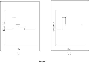
Figure 1 displays a stationary response to winning a lottery. Income will vary from the norm for a period of time. However, the response to this shock must die away in order for us to return to the same distribution. Eventually the average of income will become infinitely close to its original mean value.
As an alternative, consider that income is non-stationary. In this case, winning the lottery in a given period will cause a permanent change in average income. For example, if we could perpetuate the change in income then average income would remain higher throughout a lifetime. The shock does not to dissipate over time and the mean of income will change.
Figure 1 displays one possible non-stationary series.
The Real Business Cycle literature has dealt to a great extent with income shocks (
Kyland and Prescott, 1980). For a dynamic equilibrium to exist, we require stationarity. Otherwise, any shock to a variable will substantially change the underlying characteristics which in part determine the equilibrium value or path. We see, therefore, that our theoretical requirement for stationarity is very closely linked to the descriptive statistics and probabilistic characteristics of our data.
In Statistical Analysis
Stationarity also plays an important role in the statistical analysis of economic relationships. In order to get an accurate estimate of the coefficients determining the relationship between two or more variables, the underlying characteristics of the data series must remain constant across the sample period. Very commonly in statistical analysis, we require a series to be
second-order or weakly stationary. In second order stationarity, the mean, variance and contemporaneous covariance of the series must be constant.(
Spanos, 1986).
If
Y and
X are characterized by a normal distribution, then it can be shown that the OLS coefficients b and s2 in a simple linear regression model
Y =
b0 +
b1 +
e
are simply of combination of the means, variances of
X and
Y and the covariance of
X and
Y (
Spanos, 1994)
2. Specifically, we see that if

then
b0 = my - b1my and
b1 = s12/s2x
Therefore, the means and variances of X and Y must be constant if we can place any confidence on our estimates of b and s2.
This probabilistic interpretation of stationarity and its relationship to parameter estimation will be vital in our method of assessing parameter stability. In this paper, we will examine the assumption of stationarity by viewing the characteristics of estimated parameters, which are both theoretically interesting and functions of the joint distribution moments.
2. Graphically Examining the Stability of b Estimates
As mentioned in Section 1, the coefficients in linear regression models are simply arithmetic combinations of the moments of the joint distribution of Y and X. By varying the sample from which these coefficients are calculated, we can examine parameter properties and better understand the time invariance, or homogeneity, of Y and X.
We will consider two graphical methods to examine the properties of our Linear Regression Model (LRM) estimates. Both graphical methods can be easily implemented in a spreadsheet with limited use of specialized functions. A simple modification of formulas allows us to introduce two different methods of estimation on the same spreadsheet.
ROLS
The first graphical technique involves Recursive Ordinary Least Squares (ROLS) Regression (
Spanos, 1986). We begin by selecting a sub-sample of our data, with
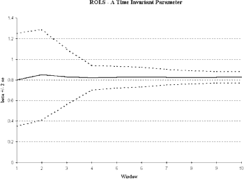
T sufficiently large, and calculating the parameters of the LRM. We find an estimate of each coefficient and the estimate’s standard error using these sub-sample observations. This process is then repeated adding one more observation to the sub-sample until the sub-sample size increases to include all the observations. If stationarity exists, we should see convergence to a stable value of the coefficient and a decreasing variance. This would indicate that additional observations bring us closer and closer to the stated value of the parameter. An example time plot of a stationary parameter is shown in
Figure 2a.
Estimation is accomplished in a spreadsheet package such as Microsoft Excel through the use of simple functions. For example, to find the estimates of the coefficients of a LRM, we type the commands:
INTERCEPT(b$1: b20, c$1: c20) and SLOPE(b$1: b20, c$1: c20)
where column b contains observations of the variable to be estimated, and column c contains observations of the regressor. The use of the dollar sign before cell 1 in each formula is crucial to the functioning of ROLS. This will enable us to copy the formulas to subsequent cells and gradually increase the number of observations used in estimation. When we copy these formulae, we have:
1
|
INTERCEPT(b$1:b20, c$1:c20)
|
SLOPE(b$1:b20, c$1,c20)
|
2
|
INTERCEPT(b$1:b21, c$1:c21)
|
SLOPE(b$1:b21, c$1,c21)
|
3
|
INTERCEPT(b$1:b22, c$1:c22)
|
SLOPE(b$1:b22, c$1,c22)
|
...
|
....
|
....
|
In this way, we have created a large number of parameter estimates, each with an increasing sample size.
An important decision regards the number of observations (20 observations here) included in the first sub-sample. There is no magic number for how many observations to include in the first sub-sample. This is only a starting point for analysis. The larger the starting sample, the more likely one is to find stationary behavior.
A similar method is used to create standard error and confidence intervals for the estimates in each sub-sample regression. The formulas in this case are more complex, but again a simple copy command with the careful use of a dollar sign enables us to form numerous ROLS estimates for the standard error and intervals. To find the standard error for the intercept term of the LRM, we must first create a column of the regressor variable squared using a simple algebra function (@c1^2). We then find the standard error of the intercept estimate is
SQRT(SUM(d$1:d20)/(COUNT(c$1:c20)*DEVSQ(c$1:c20)))*STEYX(b$1:b20,c$1:c20)
where column d contains the squares of the regressors. The standard error for the slope estimate is
STEYX(b$1:b20,c$1:c20)/SQRT(DEVSQ(c$1:c20))
Copying such formulae will result in multiple estimates of the standard errors, one for each sub-sample. An Excel algebra function can then be used to construct intervals around the estimates of each parameter. Specifically,
e$1-2f$1 AND e$1+2f$1
where column e contains the estimates of the intercept and column f contains the estimates of the standard error of the intercept estimates. These commands are copied down the column to find intervals around the point estimate for all the sub-samples.
We can then plot the estimate of each parameter (with the Insert Chart command) and its 2 standard deviation interval to examine its stationarity properties. If stationarity is an acceptable assumption, then we will find the mean of our coefficient estimate to remain nearly constant and the variance of the coefficient estimate to be shrinking. In
Figure 2a, we see a plot of a parameter that remains relatively stable and has a shrinking variance - both traits indicate homogeneity.
WOLS
Similar evidence can be displayed through Ordinary Least Squares based upon a window of observations (WOLS). In this case also, we begin with a sub-sample of our total data set. We calculate OLS estimates given this sub-sample. In order to examine the stability of these estimates, we slide this window across the entire sample, adding one observation and taking one away (Spanos, 1986). In this case, the number of observations utilized to calculate the parameters remains constant, as opposed to ROLS where the number of observations increased in each successive iteration.
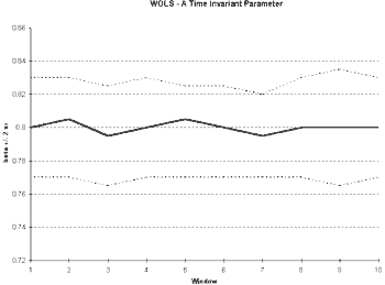
Due to this constant number of observations in the sample, we are not looking for convergence. That is, we do not expect to see a reduction in the variance. Instead, stationarity will be displayed when the estimates of the coefficients remain relatively fixed. An ideal Windows Ordinary Least Squares (WOLS) diagram would show a near constant value of the coefficient and a near constant variance (see
Figure 2b).
WOLS computation can be performed with a simple modification of the ROLS estimation spreadsheet. By removing the dollar signs in each formula and then copying the revised formulae to cells, we will create a sliding window. The formulae for the parameters INTERCEPT(b1:b20, c1:c20) and SLOPE(b1:b20, c1:c20) will become
1
|
INTERCEPT(b1:b20, c1:c20)
|
SLOPE(b1:b20, c1:c20)
|
2
|
INTERCEPT(b2:b21, c2:c21)
|
SLOPE(b2:b21, c2:c21)
|
3
|
INTERCEPT(b3:b22, c3:c23)
|
SLOPE(b3:b22, c3:c22)
|
...
|
...
|
...
|
Similar modifications of the standard error formulae allow us to construct intervals around the estimates from WOLS. In
Figure 2b, we see the behavior of a stationary parameter since the estimator’s mean and variance are relatively fixed.
 Fig 2b.
Click above to download image
3. Interpreting ROLS and WOLS Plots: An Application from Macroeconomics
As an example of studying stationarity properties in macroeconomics, we look at the relationship between consumption and income. This relationship has been explored to a great extent in the literature (see
Hall, 1989) for a survey of the historical debate). It plays a prominent role in both introductory and more advanced macroeconomics. The consumption function is also often an important application in econometrics textbooks (
Gudjarati, 1995,
Lardaro, 1993,
Ramanathan, 1998). As discussed in Section 1, non-stationarity in income would imply that a temporary change in income would lead to a persistent change in the mean and variance of that variable. To estimate and make inferences about the consumption function and to be able to speak meaningfully about the marginal propensity to consume, we must see stationarity in a statistical sense. That is, the joint distribution, D(C,Y) must display at least second order stationarity for OLS estimation to be meaningful.
We will estimate a simple linear regression model where annual consumption expenditures are a function of personal disposable income (measured in constant dollars).
3
Estimation yields:
| C = | -422.402 | | 0.936 Y, R2 = .9957 |
| (152.40) | (0.0104) |
where C is per capita consumption and Y is real per capita disposable income in the U.S. from 1959 to 1994. Next, we will examine the stability of the slope using ROLS and WOLS. In addition to providing information about the statistical reliability of our estimates, this will also display graphically patterns in the marginal propensity to consume (MPC) over time.
The Stationarity of the Marginal Propensity to Consume
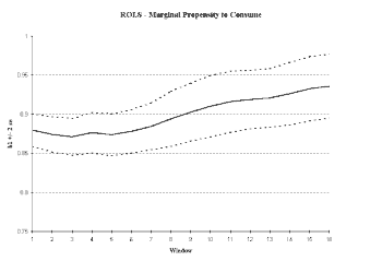
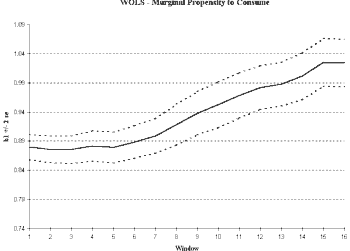
As we see from Figure 3, we have cause to doubt the stability of the parameter estimates. The initial sub-sample size in this case was selected to be 25 observations.
4 The ROLS plot in
Figure 3a shows that the MPC seems to be increasing over time. The variance in the MPC is not converging and may even be increasing as the sample size increases. Both are consistent with a non-stationary series. In the WOLS plot (
Figure 3b), we see a pronounced upward trend in the MPC with a nearly constant variance.
 Fig 3a. The ROLS plot
Click above to download image
 Fig 3b. The WOLS plot
Click above to download image
As a result, meaningful estimates of the MPC are not possible using this model. The value obtained for the MPC depends critically on the sample period selected since D(C,Y) is changing. To create a reliable estimate of MPC, we first must account for the non-stationarity.
Sources of Non-Stationarity in Theory and Application
Given our findings in the previous section, we reject the hypothesis that our parameters are time invariant or stationary.
5 However, we do not as yet know how to characterize the non-stationarity of our time series. We can identify particular types of non-stationarity with important economic interpretations. Identifying the source of non-stationarity takes us to two literature branches. First, we look at empirical models of structural change and methods to assess these drastic changes in the economy. Secondly, we consider the implications of a unit root autoregressive dynamic structure.
Structural Change
It is possible that the MPC non-stationarity results from a change in the relationship between consumption and income. For example, preferences may have changed so that a greater proportion of income is spent or saved. If this change in tastes occurs suddenly at a particular point in time, we say that a structural break has occurred.
A method of coping with non-stationarity resulting from structural change is to decrease the length of the sample in the hope that the underlying relationship is stationary over a shorter period of time (
Chow, 1960). By restricting the period of time, we may limit the amount of change in the relationship between income and consumption and therefore create a better estimate of the MPC.
To examine the stationarity of our series, we will compute ordinary least squares estimates of two sub-samples. If these coefficients vary greatly while displaying stationarity within the sub-sample, then we have shown a case for structural change. In this case an improvement in the stationarity of our series can be accomplished by viewing various sub samples. If, however, ROLS and WOLS estimates display the same non-stationarity even in the smaller samples, then we have not adequately solved this problem.
To divide our data into sub samples, however, requires the choice of a breaking point. The choice of breaking point depends upon the model in question and usually has some link to policy changes or other exogenous events. We may also use WOLS as a guide in selecting breaking points. In Figure 3, we do not notice a distinct jump in value. However, the estimates of our parameters tend to be fairly stable from the start of our sample until the mid-1980’s and then steadily increase after this time.
Estimating our Consumption function for two distinct intervals produces:
| 1959-1986: C = | 61.639 + | 0.8940 Y, R2 = .9965 |
| (133.108) | (.011) |
| 1987-1995: C = | 3153.99 + | 1.098 Y, R2 = .9288 |
| (2239.496) | (.1089) |
We see significantly different MPCs in these two intervals and that the MPC has increased in the second time period. The breaking point of 1987 is consistent with evidence from WOLS and also suggests the possible importance of tax changes in 1986. We can follow up with a standard Chow test to determine if this hypothesis of a structural break in 1986 seems valid (
Chow, 1960).
However, graphical evidence below (
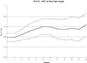
figure 4) shows that reducing the sample length does not eliminate the non-stationary behavior in MPC. While time invariance has improved, we still see an increasing MPC. Therefore, we must look for another explanation of the non-stationarity.
 Fig 4.
Click above to download image
Unit Roots
An alternative source of non-stationary behavior is a unit root autoregressive process. In this case, the value of current output depends on average upon output in the previous period. If this dependence over time does not decay b1 is equal to 1) then we see persistence of shocks and non-stationarity. This corresponds closely with the theoretical non-stationarity discussed in Section 1.
Many economists have noted the presence of numerous unit roots in economic time series including output, capital, prices and trade behavior. For a summary of these results, see
Nelson and Plosser, 1982.
If a series is unit root non-stationarity, then the estimate of b1 will be statistically indifferent from the value 1 in 6
Yt = b0 + b1Yt-1 + et
By definition, a true unit root series can be made stationary by differencing. In some cases, multiple differences may be required. This technique has been well explored in the literature on integration and cointegration (see
Dolado, Jenkinson and Rivera, 1990 for an excellent educational resource and survey.)
Next, we can examine the effect of first differences on the stationarity of the marginal propensity to consume. Forming first differences in a spreadsheet involves a simple, algebra command. The resulting columns are then used to form estimates of the LRM. With the consumption model, we find:
| 1987-1995: DC = | 60.370 + | 0.7237 DY, R2 = .626 |
| (25.430) | (.096) |
Notice the change in value of the slope term (which has changed its meaning in theory, but still captures the relationship between consumption and income) and in R2. Since this method attempts to eliminate spurious regression, we would expect to see this decrease in R2 (
Spanos, 1986).
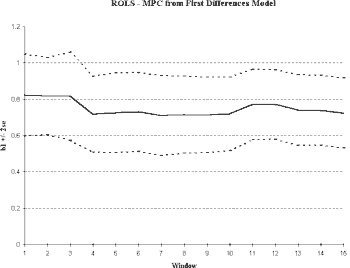
We next plot the ROLS and WOLS estimates of the slope parameter in the differenced model. As we can see in Figure 5, stationarity has been improved through differencing. We see relatively stable estimates of the relationship between consumption and income, regardless of the sample length chosen. We see a decreasing variance in ROLS indicating that additional observations improve the reliability of our estimates of the slope term. In WOLS, we find the variance remains relatively constant supporting the idea that the variance also is time-invariant. Looking at the level of integration is an important technique in construction of macroeconomic empirical models and may greatly enhance stationarity properties.
 Fig. 5a
Click above to download image
 Fig. 5b
Click above to download image
Conclusion
Stationarity of economic time series is a vital assumption in both theoretical and empirical terms. Without stationarity assumptions imposed on the first two moments of the joint distribution, we cannot justify the value of our OLS estimates. Our ordinary least squares estimates will only represent an average of various different parameter values.
This paper has demonstrated a useful approach for assessing the stationarity of an economic process and for determining if and when structural change has occurred. Dividing a sample into various sections may solve the problem of non-stationarity if the changes in the parameters result from structural change. If we see distinct changes in the parameter values, we may find we have abandoned one model for an alternative. In this case, to sample from one population only, we need to reduce the length of the sample period. However, if observed non-stationarity results from a unit root relationship, then shortening the sample period will not remove the heterogeneity. In such a case, any shock to a series will move us away from a constant mean and therefore from the assumption of stationarity. Differencing and an exploration of cointegrating vectors are necessary steps in dealing with unit roots.
Using Excel graphics enables students to see what happens to parameter estimates when a data series is non-stationary. Through exploration of data series, students can see improvements in models reconstructed to account for unit roots or structural breaks.
Notes
2. Similar reasoning applies to estimation by Method of Moments and Maximum Likelihood. Since we substitute the sample moments for population moments in Method of Moments estimation, stationarity is necessary. In Maximum Likelihood Estimation, we search for values of the parameters of the conditional distribution that will lead to the highest likelihood value. Since the likelihood function is based upon the assumed distribution, we cannot trust our estimates when the characteristics of our data change greatly throughout the sample.
3. For ease of implementation in Excel, we limit ourselves to a model with a single regressor. While it is possible to complete estimation in Excel for a case with numerous regressors (for example, using the Analysis Toolkit), this is not necessary to display both the use of statistics in macroeconomic analysis and the test for stationarity. Also, the necessary toolkit may or may not be available on the systems used by students. There are a large number of alternative models of consumption (including dynamic models with many lags, error correction models, etc.) which could be examined instead. The estimation methods for OLS, ROLS and WOLS remain very similar. However, easy spreadsheet implementation of a multivariate LRM would rely on the use of statistical functions. I often incorporate multivariate estimation of ROLS and WOLS in my econometrics course using a Matrix language like Gauss or Matlab.
4. While there is no specific rule for how large an initial sample is large enough, this size enabled us to construct 16 different estimates.
5. While this graphical analysis is a useful diagnostic tool, to reject or fail to reject a hypothesis we would need a specific test. Individuals may interpret graphs differently, and therefore we need to have some standard by which we can say that this series is “stationary enough” to call the same. Such tests have been explored in the literature on Structural change and Unit roots.
6. Since the presence of a unit root under the null will change the distribution of our estimator b1, we cannot utilize standard tests. Instead, we look to the Bootstrapped estimates of the Dickey Fuller Test (Fuller, 1976).
The author may be contacted at
Lisa A. Wilder,
Department of Economics,
Bowling Green State University,
Bowling Green
OH 43403
419-372-8397 (office);
419-353-1730 (home office);
References
Dolado, J.J., T. Jenkinson and S. Sosvilla-Rivero. 1990. “Cointegration and Unit Roots”
Journal of Economic Surveys 4: 249-273
.
Fuller, W. 1976.
Introduction to Statistical Time Series. Wiley: New York.
Gudjarati, D. 1995.
Basic Econometrics. New York: McGraw-Hill Inc.
Hall, R. 1989. “Consumption” in
Modern Business Cycle Theory, R. Barro ed. Cambridge MA: Harvard University Press.
Hall, R. 1978. “Stochastic Implications of the Life Cycle-Permanent Income Hypothesis: Theory and Evidence” Journal of Political Economy 10(2): 972-987.
Hamilton, J. 1994.
Time Series Analysis. Princeton NJ: Princeton University Press.
Judge, G. 1990.
Quantitative Analysis for Economics and Business Using Lotus 1-2-3. Hemel-Hempstead: Harvester-Wheatsheaf.
Kyland, F. and E. Prescott. 1980. “A Competitive Theory of Fluctuations and the Feasibility and Desirability of Stabilization Policy” in
Rational Expectations and Economic Policy, S. Fisher ed. Chicago : University of Chicago Press.
Lardaro, L. 1993.
Applied Econometrics. New York: Harper Collins Publishers.
Nelson, C.R. and C.I. Plosser. 1982. "Trends and Random Walks in Macroeconomic Time Series"
Journal of Monetary Economics 10: 139-162.
Paetow, H. 1994. “Illustrating Microeconomic Theory by using Spreadsheets”
Computers in Higher Education Economics Review 22.
Ramanathan, R. 1998.
Introductory Econometrics with Applications. Fort Worth, TX: The Dryden Press.
Spanos, A. 1994.
An Introduction to Modern Econometrics. Cambridge: Cambridge University Press.
Spanos, A. 1986.
Statistical Foundations of Econometric Modelling. Cambridge MA: Cambridge University Press.
United States Department of Labor, Bureau of Labor Statistics, 1998. Consumption and Disposable Personal Income, 1959-1994.
Whitmarsh, D. 1991. “A Spreadsheet Model of Renewable Resource Exploitation”
Computers in Higher Education Economics Review 13.

